
Design and development of subsystems
Step one – choice of the architecture (structure).
The standard proposes four predefined architectures and for each of them provides a simplified formula for computation of the PFH.
The four architectures are differentiated by the hardware fault tolerance (HFT), and for the presence (or absence) of diagnostics.
The four architectures correspond to the most popular configurations used in the field of safety of machinery.
A hardware fault tolerance of N means that the subsystem tolerates up to N failures before losing his safety performance. N +1 faults could cause a loss of the safety function.
When defining the fault tolerance of an architecture no credit is given to additional measures that can control the effects of faults, such as diagnostics.
For architecture B and D the two channels are sufficiently independent; i.e. they are designed in such a way that a single channel is able to carry out the function independently from the other. The same apply to the architecture C for the functional channel with respect to the diagnostic channel.
Subsystem architecture A:
HFT = 0 – Single channel without diagnostic function

Fig. 17 – Basic subsystem architecture A
Any dangerous failure of a subsystem element causes the loss of the safety function.
(1) PFH = λDe1 + ….. + λDen
Where:
λDei is the dangerous failure rate of an element of the single channel.
Cat. B (PLmax = b)
Cat. 1 (PLmax = c)

Subsystem architecture B
HFT = 1 – Dual channel without diagnostic function
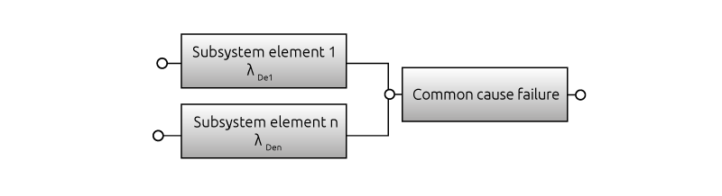
Fig. 18 – Basic subsystem architecture B
A single failure of any subsystem element does not cause a loss of the safety function
(2) PFH = (1 – β )2 x λDe1 x λDe2 x T1 + β x ( λDe1 + λDe2) /2
Where:
λDe1 is the dangerous failure rate of an element of the first functional channel
λDe2 is the dangerous failure rate of an element of the second functional channel
T1 is the useful lifetime or the proof test interval, whichever is the smaller.In anycase not exceeding 20y
β is the susceptibility to common cause failures.
No correspondence with the categories of EN ISO 13849-1
Subsystem architecture C:
HFT = 0 Single channel with a diagnostic function
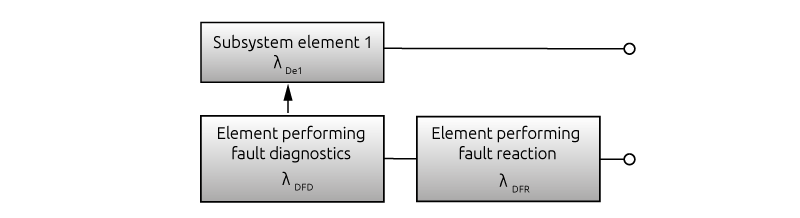
Fig. 19 – Basic subsystem architecture C
Any undetected dangerous fault of a subsystem element of the functional channel leads to the loss of the safety function. When a dangerous fault of a subsystem element of the functional channel is detected by the diagnostic function, the diagnostic function itself initiates a fault reaction.
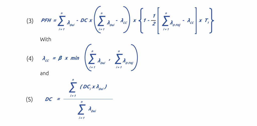
Where:
T1 is the useful lifetime or the proof test interval, whichever is the smaller. In any case not exceeding 20y
λDei is the dangerous failure rate of element ei within the single functional channel.
n is the number of elements of the single functional channel.
λDFHj = λDFDj + λDFRj is the failure rate of the elements number j within the single channel that realizes the fault handling function.
m is the number of elements of the single channel that realizes the fault handling function(s)
DCi is the diagnostic coverage for element ei of the single functional channel.
β is the susceptibility to common cause failures of the functional channel and of the diagnostic channel.
If the diagnostic function is performed by a separate subsystem within the SCS,
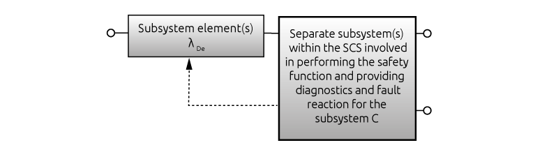
Fig. 20 – Separate subsystem within the SCS
Then
λD FH j = 0
β < 2%- due to the separation of the two subsystems and the equations simplify to
(6) PFH = ( 1- DC1 ) x λDe1 + … + ( 1 – DCn ) x λDen
The test rate of the diagnostic functions must be at least a factor of 100 higher than the demand rate of the safety function and the time needed for the fault reaction must be short to bring the system to a safe state before a hazardous event occurs.
Alternatively, the test can be performed periodically. In this case the sum of the test interval, plus the time needed to detect a fault plus the time needed to bring the system to a safe state is shorter than the process safety time.
The test can also be performed immediately upon any demand of the safety function. In this case the time needed to detect a fault and to bring the system to a safe state must be shorter than the process safety time.
Cat. 2 (PLmax = d)

Subsystem architecture D
HFT = 1 Dual channel with a diagnostic function
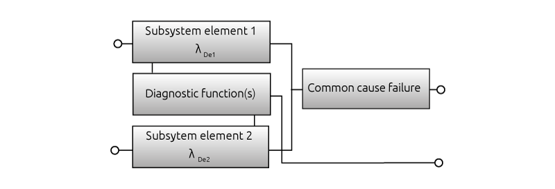
Fig. 21 – Subsystem architecture D
For subsystem elements of the same design:
(7) PFH = (1-β ) 2 x [DC x T2 + (1-DC) x T1 ] x λDe2 + β x λDe
For subsystem elements of different design
(8) PFH = (1-β)2 x [λDe1 x λDe2 x (DC1 + DC2 ) x T2 /2 + λDe1 x λDe2 x (2-DC1-DC2 ) x T2 /2 +β x (λDe1 x λDe2) / 2
Where
T2 is the diagnostic test interval.
T1 is the useful lifetime or the proof test interval, whichever is the smaller. In any case not exceeding 20y
β is the susceptibility to common cause failures
λDe1 is the dangerous failure rate of subsystem element 1
λDe2 is the dangerous failure rate of subsystem element 2
DC1 is the diagnostic coverage for subsystem element 1
DC2 is the diagnostic coverage for subsystem element 2
A single dangerous fault of any subsystem element does not cause a loss of the safety function. Where a fault of a subsystem element is detected by the diagnostic function, the diagnostic function itself initiates a fault reaction.
The diagnostic function is performed continuously, and the sum of the diagnostic test interval and the time needed to perform the specified fault reaction, in order to bring the system to a safe state, must be shorter than the process safety time.
Cat. 3 (PLmax = d)
Cat. 4 (PL = e)

Step two – determination of the parameters λ, λd, λs, λdd, λdu
General considerations
For purpose of determining the failure rates of subsystem elements, the following fault criteria shall be considered:
- If, because of a fault, further components fail, the first fault together with all following faults shall be considered as a single fault
- Two or more separate faults having a common cause shall be considered as a single fault
- The simultaneous occurrence of two or more faults having separate causes is considered highly unlikely and therefore need not be considered
- Certain faults may be excluded, provided that the likelihood of them occurring is very low in relation to the safety integrity requirements of the subsystem
A basis for fault consideration is given in ISO 13849-2 (Annexes A to D).
For the list of components/elements included in Annexes A to D, are provided:
- The faults to be considered
- The permitted fault exclusions, considering environmental and application aspects and conditions under which fault exclusion are permitted
Electrical/electronic components
Determination of λ
In general, for this type of components the manufacturer does not provide reliability data because they strongly depend on how the component is used and on the characteristics of the environment.
Reliability data can be found in the set of standards SN 29500 or in the MIL-HDBK 217F or OREDA 2015 or even in the EXIDA reliability handbook.
Failure rates are expressed in FIT (failure in time).
1 FIT = 1 x 10⁻⁹ hours
FIT values are given at reference operating conditions (voltage, current, dissipation etc..) and at the ambient temperature of 40 ° C. The value given is λref in FIT.
Example: for a metal fil resistor is λref = 0,2 FIT
If the actual operating conditions are different respect to the reference ones, it is necessary to make corrections using formulas that are provided in the same document for each family of components.
Determination of λd and λs
After having determined λ for each subsystem element (e.g. derived by one of the data base mentioned), the different failure modes of the subsystem element should be considered. It is typically assumed that not all failures modes lead to a dangerous failure. To determine the failures to consider for each element and to decide whether they are safe failures or dangerous failures, an analysis technique, such as failure mode and effect analysis (FMEA) or fault tree analysis (FTA) should be carried out.
In order to undertake this technical analysis, the following information is necessary:
- The hardware schematics of the subsystem describing each component and interconnections between components
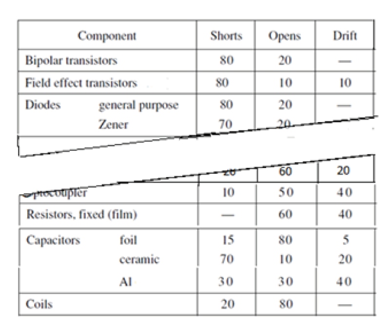
- For each component the failure modes and associated percentages of the total failure probability
To help the designer, several recognised industry sources are available where to find a list of failure modes together with the failure mode ratio.
The process should be as follows:
Categorize each failure mode according to whether it leads to
- A safe failure (fault has no influence or the fault leads to a safe state without a diagnostic measure
- A dangerous failure (leads without diagnostic to a dangerous malfunction)
- Components that are not a part of a safety function or of a diagnostic measure, and that do not have any influence on the safety function are not considered.
Doing this analysis, do not consider the effects of diagnostic techniques implemented! The effects of diagnostics are considered separately; see the clause: computation of DC.
From the estimate of λ of each component and the categorization of the failures (safe, dangerous) calculate the probability of safe failure (λS) and the probability of dangerous failure (λD)
Example, just to describe how to apply the method:
Let’s take for ease of computation the case of two components, a ceramic capacitor and a metal film resistor that are part of the components of a functional channel.
For the capacitor we get from SN 29500 a failure rate of 2 FIT (λ = 2 x 10⁻⁹). From the analysis of the circuit, it comes that a short circuit of the capacitor or a drift leads to a dangerous failure, while an open circuit leads to a safe failure.
For the resistor we get from SN 29500 a failure rate of 0,2 FIT (λ = 0,2 x 10⁻⁹). From the analysis of the circuit, it comes that an open circuit of the metal film resistor or a drift leads to a dangerous failure, a short circuit leads to a safe failure, but this type of failure for a metal film resistor is excluded, due to the technology. (see ISO 13849-2).
For the capacitor:
λScap = 2 x 10-9 x 0,1 = 2 x 10⁻¹⁰
λDcap = 2 x10-9 x (0,7 + 0,2) = 1,8 x 10⁻⁹
For the resistor:
λDres = 0,2 x10-9 x (0,6 + 0,4) = 0,2 x 10⁻⁹
Obviously, the same calculations must be carried out for all components of the channel.
The overall values of λS and λD for the channel are then derived by summing the values of λS and λD of each components.
Limited to the components of our example:
λSchannnel = 2 x 10⁻¹⁰
λDchannel = 1,8 x 10⁻⁹ + 0,2 x 10-9 = 2 x 10⁻⁹
Alternative method:
If no specific information is available concerning the failure modes, 50 % of the failures can be estimated as dangerous, in this case λS and λD are approximated to:
For the capacitor:
λScap = 2 x 10-9 x 0,5 = 1 x 10⁻⁹
λDcap = 2 x10-9 x (0,5) = 1 x 10⁻⁹
For the resistor:
The technology used excludes the fault of short circuit; if no additional information is available, all the other faults must be considered dangerous:
λDres = 0,2 x10⁻⁹
Determination of λd for electromechanical components
For electromechanical, pneumatic and mechanical components subject to wear (eg. relay and solenoid valves) the failure rate increases with the number of cycles processed.
For this reason, their reliability is usually related to the number of cycles performed and not to the time for which they have been working.
The parameter given by the manufacturer is the B10 or the B10d expressed in numbers of operations; this is the number of operations after which failures occur in 10% of the components tested (endurance test under specified load).
If manufacturer data are not available, for a list of hydraulic, pneumatic, and electromechanical components, it is also possible to use the B10d or MTTFd values given in Table C.1 of the standard. The use of these values is allowed only under the following conditions:
- Basic and well-tried safety principles according to ISO 13849-2 have been used for the design of the component (confirmed in the data sheet of the component)
- The manufacturer of the component specifies that the component can be used for safety related applications
- The subsystem designer confirm that the component is utilized fulfilling basic and well-tried safety principles according to ISO 13849-2.
Hydraulic components listed in Table C.1 are characterized with MTTFd. For the conversion of MTTFd into a λd value the following basic equation can be used:
(9) λd= 0.1 / MTTFD x 8760 h/a
Note: MTTFd is given in years; one year is approximatively 8760 hours
For the conversion of B10d into a λd value the following equation can be used:
(10) λd= (0.1 X C) / B10d
Where:
C = nop / 8760 (mean number of operations per hour)
The operating time of the component must then be limited to T10d which is the average time within which 10% of the components undergoes a dangerous failure.
(11) T10d = 0,1 / λd
If only B10 is available (the number of operations after which 10% of the components under test undertake a failure), B10d can be derived knowing the ratio of dangerous failures (RDF)
(12) B10d = B10 / RDF
If no other information is available, RDF is estimated as 0,5 (50 % dangerous failure).
For a low duty relay the manufacturer specifies a B10 = 10 M cycles when used at small load (20% of the nominal load).
The relay is used on a machine operated as follows:
220 days/year; 16 h/day (two shifts); machine cycle: 1 min (60 cycles/h)
From the above formulas it comes:
Mean number of annual operations nop = 211200
Mean operation per hour C = 24,11 /h
No information is given regarding B10d, therefore is assumed B10d = 2 x B10
then: λd = 0,1* 24,11 / 20*106 = 1,2*10-7/h
A more precise analysis can be carried out by retrieving from a reliability data base the list of failure modes and failure mode ratios of the relay and analysing, for the given application, which are the dangerous failures:
Example:
| Component | Failure mode | Typical failure mode ratios % | |
| Relay | All contacts remai in the energized position when the coil is de-energized | 25 | D |
| All contacts remai in the de-energized position when the coil is energized | 25 | S | |
| Contact will not open | 10 | D | |
| Contact will not close | 10 | S | |
| Simultaneous short circuit between three contacxts of a change-over contact | 10 | D | |
| Simultaneous closing of normally open and normally closed contact | 10 | D | |
| Shor circuit between two pairs of contacts and/or between contact and coil terminal | 10 | D | |
Ratio of dangerous failures (RDF) = 65%
From equation : B10d = 10M / 0,65 = 15,38 M operations
Then λd = 0,1* 24,11 / 15,38*106 = 1,57*10-7/h
Step 3 – Determination of Diagnostic Coverage (DC) and of the parameters λdd and λdu
Assuming that
- A failure can always happen (otherwise there would be no reason to define λ)
- Is not possible to detect all faults because the mechanisms for the detection of faults are not all equally effective and immediate (for some faults may take longer)
- But taking appropriate diagnostic measures most of the dangerous faults can be detected
it is possible to define a parameter DC which gives an estimate of the efficiency of the diagnostic measure implemented.
DC is defined as the ratio between the failure rate of dangerous failures detected (λdd) compared to all dangerous failures detected and not detected (λd).
(13) DC = λdd / λd
Calling λdu the fraction of dangerous failures that remain undetected it comes that
(14) λd = λdd + λdu
And:
(15) λdd = λd x DC
(16) λdu = λd x (1- DC)
IEC 62061 provides a list of different diagnostic techniques in Annex D and for each of them a parameter DC is given representing the fraction of dangerous failures that can be detected by the application of that diagnostic technique.
DC range is from 0% to 99%
DC = 0% representing no dangerous fault is detected
DC = 99% representing very high fraction of dangerous faults detected
The designer must select for each subsystem element, the diagnostic technique that would be better suited to its application (for input signals, for processing logic, for the outputs) and at the same time ensuring the DC level needed.
Example: if the diagnostic measure implemented for the control of dangerous failures of the relay of the previous example is implemented by monitoring the functioning of the relay by a mechanically linked NC contact, from Table D.1 it follows DC = 99%:
Then
λdd = 1,2 x 10-7 x 0,99 = 1,188 x 10-7
λdu = 1,2 x 10-7 x 0,01 = 1,2 x 10⁻⁹
The overall Diagnostic coverage DC of a subsystem is:
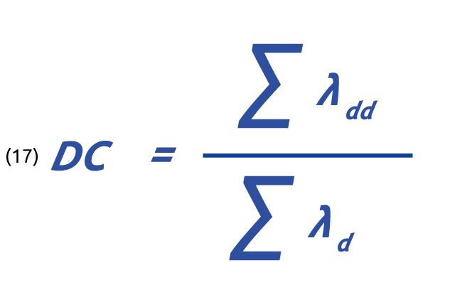
where
∑ λdd is the sum of the rate of dangerous failures detected of all subsystem elements and
∑ λd is the sum of the rate of dangerous failures of all subsystem elements
Realization of diagnostic functions
The diagnostic functions are considered as separate functions that may have also a different structure than the SCS and may be performed by:
- The same subsystem which requires diagnostics
- Or subsystems of the SCS not performing the SCF
- Or other subsystems of the SCS
Example of diagnostic function of type c)
The SCS is made of two subsystems:

Subsystem 1 is a photochell with an MTBF = 10 years (emitter + receiver)
Subsystem 2 is an AU SX safety control unit SIL 2 rated with a PFH = 5 x 10⁻⁹
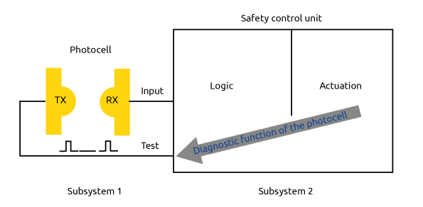
Diagnostic measure selected: online monitoring with check of the response time of the Photocell
From Table D.1: Cyclic test stimulus by dynamic change of the input signals DC = 90%.
Subsystem 1:
For calculation purposes, MTBF can be assumed equal to MTTF,
The ratio of dangerous failures is estimated as 0,5, therefore
MTTFd = 2 x MTTF
λd = 5,7 x 10⁻⁶
HFT = 0 (architecture C)
β ≤ 2%
As the diagnostic function is performed by the separate subsystem 2 within the SCS, formula (PFH = ( 1- DC1 ) x λDe1 + … + ( 1 – DCn ) x λDen) can be applied for the estimation of the PFH:
PFH (subsystem 1) = (1-DC) x 5,7 x 10-6 = 5,7 x 10⁻⁷
The overall PFH of the SCS is: PFH (scs) = 5,7 x 10⁻⁷ + 5 x 10-9 = 5,75 x 10⁻⁷
Step 4- Estimation of safe failure fraction
After having derived for each subsystem the PFH it is important to ensure that the associated SIL is compatible with the limitations imposed by the architecture. The highest safety integrity level that can be claimed for subsystem is limited by the safe failure fractions (SFF) as specified in the following table
| Safe failure fraction (SFF) | Hardware fault tolerance | ||
| 0 | 1 | 2 | |
| SFF < 60% | Not allowed | SIL 1 | SIL 2 |
| 60% ≤ SFF < 90% | SIL 1 | SIL 2 | SIL 3 |
| 90% ≤ SFF < 99% | SIL 2 | SIL 3 | SIL 3 |
| SFF ≥ 99% | SIL 3 | SIL 3 | SIL 3 |
Subsystem safe failure fraction (SFF) is, by definition, the fraction of the overall failure rate that does not result in a dangerous failure.
It is therefore the ratio between the sum of the overall safe failures and dangerous failures detected by the diagnostic techniques implemented and the sum of all possible failures (safe, dangerous detected and dangerous not detected).
(18) SFF = (Σλs + Σλdd) / Σλs + Σλd
For the calculation, all the components including electrical, electronic, electromechanical, mechanical etc, which are necessary to allow the subsystem to process the safety function shall considered.
Methodology for the estimation of susceptibility to common cause failures
In case of redundant structures, the methodology used for calculating the PFH assumes a sufficient operating independence of the two channels.
However, if the channels are not fully independent, common cause failures due to a single occurrence or condition can cause a critical malfunction simultaneously on both channels in a dual channel architecture.
Examples of failures due to common causes such common-cause faults are:
- Power surges (a surge strong enough to cause multiple catastrophic failures one channel will likely destroy the other at the same time)
- Impurity of the fluid medium (valves of both channels fail to open)
- Overtemperature (due to a failure of the cooling fans).
Estimation of the effect of CCF
The likelihood of common cause failure introduces the problem of estimating the rates of simultaneous failure for multiple components in addition to their Individual failure rates.
IEC 62061 overcome this problem by using the scoring method proposed in Annex E.
Table E.1 of this Annex gives a list of measures and for each measure an associated values is assigned which represent the contribution of each measure to the reduction of common cause failures.
All the factors having an impact on the design of the subsystem must be added to provide an overall score.
For each listed measure, only the full score or nothing can be claimed.
If a measure is only partly fulfilled, the score according to this measure is zero.
Where it can be shown that equivalent means of avoiding of CCF can be achieved through the use of specific design measures (e.g. the use of opto-isolated devices rather than shielded cables), then the relevant score can be claimed as this can be considered to provide the same contribution to the avoidance of CCF.
If equivalent means of avoiding of CCF can be achieved through the use of specific design measures (e.g. the use of opto-isolated devices rather than shielded cables), then the relevant score can be claimed.
The overall score is used to determine the common cause failure factor β from table F.2 as a percentage value.
Overall score | Common cause failure factor (β) |
≤ 35 | 10% (0,1) |
36 to 65 | 5% (0,05) |
66 to 85 | 2% (0,02) |
86 t0 100 | 1% (0,01) |
This β factor will be used in formulas 2, 4, 7, 8 for the calculation of the PFH of a subsystem.

