
Choice of self-diagnosis techniques and DC computation
If it is supposed:
- That a failure can always occur (otherwise there would be no reason to define the MTTF)
- That the mechanisms for faults detection are not all equally efficient and immediate (it depends on the type of fault, for some faults it may take longer time) and that it is not possible to be able to detect all faults
- However, by adopting suitable circuit arrangements, it is possible to detect most of the dangerous faults
Then it’s possible to define a DC parameter that specifies how efficient the system is in detecting its own malfunctions “in time” (in time means before a second dangerous fault can occur).
DC computation – General rule
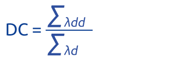
The DC parameter is expressed as the ratio between the failure rate of dangerous failures detected by the implemented self-diagnostic measures, λdd, and the failure rate of all possible dangerous failures λd (detected and undetected).
Knowing λd and the percentage of fault coverage provided by the diagnostic measures implemented, it is possible to derive λdd (detectable) and λdu (not detectable) and then compute the value of DC for the entire subsystem.
DC computation – Simplified method
This simplified method is based on the diagnostic techniques listed in Table E.1 of the Standard. Table E: 1 provides a list of 34 different diagnostic techniques divided into three families (for input circuits, for processing logic, for output circuits). If the designer decides to use diagnostic techniques to increase fault coverage, he can choose the preferred techniques among those listed in Table E.1 that best suit its application. A variable fraction of DC coverage ranging from0% to 99% is assigned to each technique.
- 0% = the selected technique does not detect dangerous faults
- 60% = a low fraction of dangerous failures is detected
- 90% = an average fraction of dangerous failures is detected
- 99% = a very high fraction of dangerous failures is detected
It is also possible to select diagnostic techniques with different DC values for the individual parts. The formula that allows the computation of the DC of the entire system (DC) is
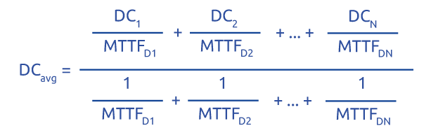
Where MTTFDi and DCN are the values of MTTFD and DC of the individual components of the subsystem
A component with a low DC and a low MTTFD has great weight and leads to a low DC value. A part that is not tested gets a
DC = 0 and contribute only to the value of the denominator. Once the calculation is completed, a DC class is chosen by means of the following table:
As was done for the choice of the MTTFD, also for the DC the Standard does not require knowledge of the exact value for the computation of the PFHd, but that a choice is made among four ranges of values.
| Denomination DC | Range of values DC |
None | DC < 60% |
Low | 60% ≤ DC < 90% |
Mediun | 90% ≤ DC < 99% |
High | 99% ≤ DC |

